GUI Overview
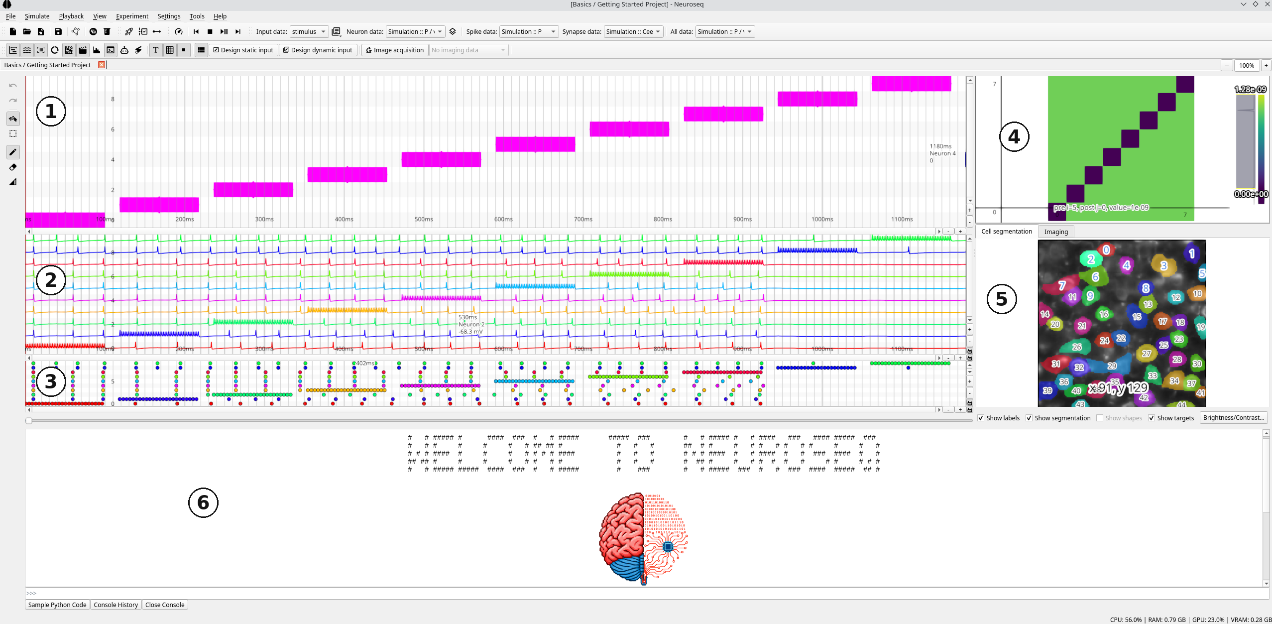
Panels: input array editor (1), traces (2), spikes (3), synapse heatmap (4), Cell segmentation and Imaging tabs (5) and console (6). The Custom Analysis panel opens when you run an analysis. Show or hide each with View → Show … or the View toolbar (Show Data is the All data panel). Right-click a panel for Detach panel or Detach copy of panel (e.g. to compare two time windows).
Project tabs
Each project opens in its own tab (New, Open Project, an example
project, or a dropped .nseq). Menus and toolbars act on the current tab.
Closing a tab with unsaved changes asks to save. Only one simulation can run
at a time across all tabs.
Menus
| Menu | Contents |
|---|---|
| File | New (Ctrl+N), Open example project, Open Project (Ctrl+O), Import from Project, Cell segmentation, Save Project (Ctrl+S), Save Project As..., Import data, Export, Edit Model (Ctrl+E), Generate Synthetic Data... (Ctrl+G), Manage Data |
| Simulate | Run Simulation (Ctrl+R), Store / Restore Simulation Checkpoint (Ctrl+Shift+S / Ctrl+Shift+R) |
| Playback | Set Playback Speed, Skip to Start, Stop (pause and rewind), Play / Pause (Space), Skip to End |
| View | Show panels, Toggle Selection Text, Toggle Grid, Keep Short Inputs Visible (4 px), Show all input arrays |
| Experiment | Connect (Brian2) External Input Function, Run External Input Function (external simulators) |
| Settings | See below |
| Tools | Open Fiji, Open Cellpose, Change Fiji Path… |
| Help | Documentation (F1), Source Code, About |
Import and export
| Path | Purpose |
|---|---|
| Import data → Input → Optogenetics | SysCon2 .seq (holographic stimulation) |
| Import data → Input → Patch Clamp | Igor2 .ibw/.pxp or .csv/.txt input waves (patch-clamp data) |
| Import data → Output → Calcium Imaging (raw .tif) | raw 2-photon TIFF via Cellpose + Suite2p (imaging data) |
| Import data → Output → Calcium Imaging (Suite2p outputs) | existing Suite2p results |
| Import data → Output → Patch Clamp | recorded traces |
| Export → Patch Clamp Input | input for SutterPatch (patch clamp export) |
| Export → Optogenetic Input | SysCon2 .seq files only. To also load them into a connected SysCon2, use Export with settings… in the Stimulation setup pane. |
| Export → Traces / Spikes as NumPy Array… | array of neurons × time (see below) |
NumPy export: traces keep their own samples at full resolution. Spikes are
counted per bin; the bin defaults to the frame period of a trace in the same
data group, else 1 ms. .npy holds only the array; .npz also holds
neuron_ids, times (s) and units, with the array as values.
File → Manage Data lists data groups and their data sets to rename, describe or delete them.
The file dialogs of the data imports (cell segmentation, calcium imaging, Suite2p, patch clamp, SysCon2) open in the folder that project used last, so each open project tab keeps its own folder. A project that has none yet starts in the folder used last in any project. The folder is saved with the project.
Dropping files
Dropped files open their usual import dialog, prefilled:
| File | Dropped on | Import |
|---|---|---|
.nseq |
anywhere | project, in a new tab |
.seq |
anywhere | SysCon2 sequence as an input array |
.ibw, .pxp, .csv, .txt |
input array editor | patch-clamp input wave |
.ibw, .pxp, .csv, .txt |
anywhere else | patch-clamp traces |
| TIFF or PNG | Cell segmentation tab | cell segmentation, file ready to segment |
| TIFF | traces, spikes or All data panel | calcium trace extraction |
| TIFF, GIF or movie | Imaging tab | imaging data |
| TIFF, PNG, GIF or movie | anywhere else | asks which of the three imaging imports |
Saving and undo
- Save Project (
Ctrl+S) writes back to the current.nseqwith no dialogs. Save Project As... picks a new file and which components to include. A never-saved project always goes through Save As. - Open and save run in the background with a cancellable progress dialog. Cancelling a save leaves the original file untouched.
- Undo (
Ctrl+Z) / Redo (Ctrl+Shift+Z) cover input-array edits, imports and renames, descriptions and deletions in Manage Data. History is per tab and not saved in the file.
Data toolbar
Comboboxes select what each panel shows: Input data, Neuron data, Spike data, Synapse data and All data (a universal panel for any traces or spikes). The button next to Input data opens array operations: create, edit, delete, clear, Trim to Mapped Neurons…, pad, trim, loop. Overlay input on traces draws the selected input array behind the Neuron data traces (each neuron's input on its own trace row) and hides the input editor. Overlay input on All data traces, next to the All data selector, does the same for the All data panel when it shows traces, for example a second calcium trace array, and leaves the input editor where it is. Each trace view, including detached panels, switches its overlay on and off on its own: right-click the traces and choose Overlay input on traces. A detached copy starts with the setting of the panel it was copied from. Every overlay follows the Input data selector and redraws after input edits, undo and redo.
The View toolbar also holds Design static input, Design dynamic input (input design), Image acquisition (ScanImage controls) and the Imaging tab's data selector.
Navigation
- Pan: scrollbars, mouse wheel (vertical) or middle-button drag. Panels are linked by default.
- Zoom: +/− buttons,
Ctrl+wheel (time),Shift+wheel (neurons). - Toggle Selection Text hides the coordinate label at the cursor. The label shows the neuron and its value at the cursor time (traces: the nearest sample, with that sample's time). Times on the axis, the label and selections use seconds when 2 s or more are visible and milliseconds otherwise, with more decimals the further you zoom in.
- Toggle Grid shows a time/neuron grid on the input editor, spaced by the
array's
dt. - Right-click the traces for Normalization… (percent scale, Center median, Clip values, Auto-extend vertical space), Overlay input on traces and Preview vector graphic…. The synapse heatmap has its own Normalization….
Comparing trace arrays
Repeats of the same input give several trace arrays. To compare them without switching the Neuron data selector back and forth, right-click the traces and choose Compare traces…:
- Tick any number of Neurons. The selected neuron range (or the neuron
under the cursor) is ticked already. Filter the list by id or range
(
10-20); Select all/Select none act on the neurons the filter shows, and the field below ticks a list such as0-5, 9. - Tick the Trace arrays to compare. Every trace array of the project is listed; the one the trace view shows is ticked. Drag the arrays, or use Up/Down, to set their order (it matters for Concatenated).
- Choose a View:
- Overlay per neuron: one row per neuron, overlaying that neuron's trace from every chosen array, each array in its own colour as named in the legend.
- Side by side per neuron: the same rows, but every array gets its own column. The window's Side by side box switches between these two.
- Separate window per array: one window per array, each showing the chosen neurons stacked one row per neuron. With Lock time axis (on by default), zooming or panning time in one window moves every other locked window; Lock value axis (off by default) does the same for each neuron's value range. Every window has its own lock boxes, so you can unlink a window later (ticking a box again snaps it back to the others). The windows open fanned out so they don't cover each other completely; closing one leaves the others linked.
- Concatenated: the arrays joined end to end, in the list's order, into one long timeline per neuron. Each segment is drawn in its array's colour on its own sampling interval, starting where the previous one ended (plus the optional Gap). Dashed lines mark the boundaries and the array names label the segments.
OK opens the window(s); you can keep several open. All rows of a window share one time axis, so zooming or panning one (toolbar above the plot) moves them all. Each array is drawn on its own time axis, so arrays with a different sampling interval or length still line up in time. A neuron missing from an array is skipped there (left empty in the concatenated view), and a note at the top lists which. The windows only read the data: they change nothing in the project and add no undo step.
The one exception is Also add as new trace array to the project under
Concatenated. It stores the joined traces of the ticked neurons as a new
data group, named in the Name field (Concatenated: Rep 1 + Rep 2 + … by
default), which then appears in the data selectors. Neurons missing from an
array and the gap are filled with NaN. Adding is one undo step (Undo removes
the array again). It is only offered when every ticked array has the same
sampling interval; otherwise the box is disabled and its tooltip lists the
arrays' intervals.
Input editor
The left toolbar has Undo/Redo, Draw mode (1) and Select mode (2).
- Draw mode: left-click draws, right-click erases (inverted in Erase input). Hold to draw longer. Set input value/length… sets amplitude (Constant or Ramp) and duration. Opacity shows amplitude relative to the array maximum.
- Select mode: select all, copy, cut, paste, paste inverted, save/load region to file, delete region.
- Show all input arrays draws the other arrays faintly behind the current one.
Details: static input.
Cell segmentation and Imaging tabs
The Cell segmentation tab shows Cellpose cells labelled with neuron ids, each in the same colour as that neuron's traces, spikes and inputs:
- Left click: select or deselect a cell. Traces, inputs and spikes then show only selected neurons.
- Right drag: lasso several cells. Double-click empty space: clear selection.
- Right click a cell: scroll the traces to its neuron (if visible).
The Imaging tab plays imported imaging movies.
Stimulation setup
View → Show Stimulation setup has one tab per target: SysCon2 (HOLO4D) (holographic stimulation), BrainScaleS-2 (BrainScaleS-2) and ScanImage (imaging) (ScanImage acquisition).
Synaptic data widget
The Heatmap panel shows the synaptic weight matrix of the selected Synapse data at the playback time. Above Settings → Synapse Matrix RAM Limit it downsamples in time.
Analysis
Select a region in the traces, right-click and pick an analysis. Results appear in the Custom Analysis panel, or in a new window if Open analysis in a new window is checked. See analysis and plugins.
Settings
| Setting | Effect |
|---|---|
| Brian2 Simulation Backend | numpy (default) or cython (simulations) |
| Input Automatic Padding | seconds of empty input added after each run (default 0) |
| LLM Assistant | provider, model, key and data scope |
| Synapse Matrix RAM Limit | MB before the synapse heatmap downsamples (default 256, 0 = no limit) |
| Trace Plot RAM Limit | same for trace plots (default 256) |
| Theme | Light, Dark or Retro light theme (beta) (default); remembered across launches |
Console
A Python console at the bottom of the window. Namespace: np, b2, plt
(matplotlib) and project. Up/down arrows browse history; Console History
lists it and Sample Python Code shows copyable snippets.
>>> project.stim_arrays.keys()
>>> project.stim_arrays['stimulus'].values[::10, ::2] = 1
>>> for i in range(10):
...     project.stim_arrays['stimulus'].values[i*10:(i+1)*10, i] = 1
>>> project.b2_model.monitors.keys()
>>> monitor = project.b2_model.get_monitor('trace')['object']
Direct writes to values are not undoable; use
project.replace_stim_values(name, values) for an undoable edit. Read Brian2
objects but do not modify them, or the GUI gets out of sync. See
help(project.b2_model).